Basics of Bayesian modelling

Background

Bayesian inference is a method of statistical inference in which we use probability to expresses a degree of belief or uncertainty about the parameters in our statistical model. It updates beliefs in light of new data using Bayes’ Theorem.

Bayes theorem

For a parameter \(\theta\) and data \(D\), Bayes theorem is:

\[ p(\theta|D) = \frac{p(D|\theta)p(\theta)}{p(D)} \]

• \(p(\theta)\) is the prior - our belief about \(\theta\) before seeing the data
• \(p(D|\theta)\) is the likelihood - how likely the data is given \(\theta\)
• \(p(D)\) is the marginal likelihood (evidence) - an overall measure of the probability of the data
• \(p(\theta|D\) is the posterior - puts it all together to give a updated probability of \(\theta\) given \(D\).

Step by step example

Data

Our data generating process is:

\[y = f(x;\theta) + \epsilon, \epsilon \sim \mathcal{N}(0,\sigma^2)\] We’ll consider a linear univariate case where \(f(x;\theta)=\theta \cdot x\) where \(\theta=1.2\):

data_sim <- function(n=100,theta=1.2,s=1.0) {
  x <- rnorm(n)
  e <- rnorm(n,sd=s)
  y <- theta * x + e
  data.table(x = x, y = y)
}

Generating \(n=100\) samples for our example:

set.seed(1234)
D <- data_sim()
ggplot(D,aes(x = x, y = y)) +
  geom_point() +
  labs(title = "Observed sample")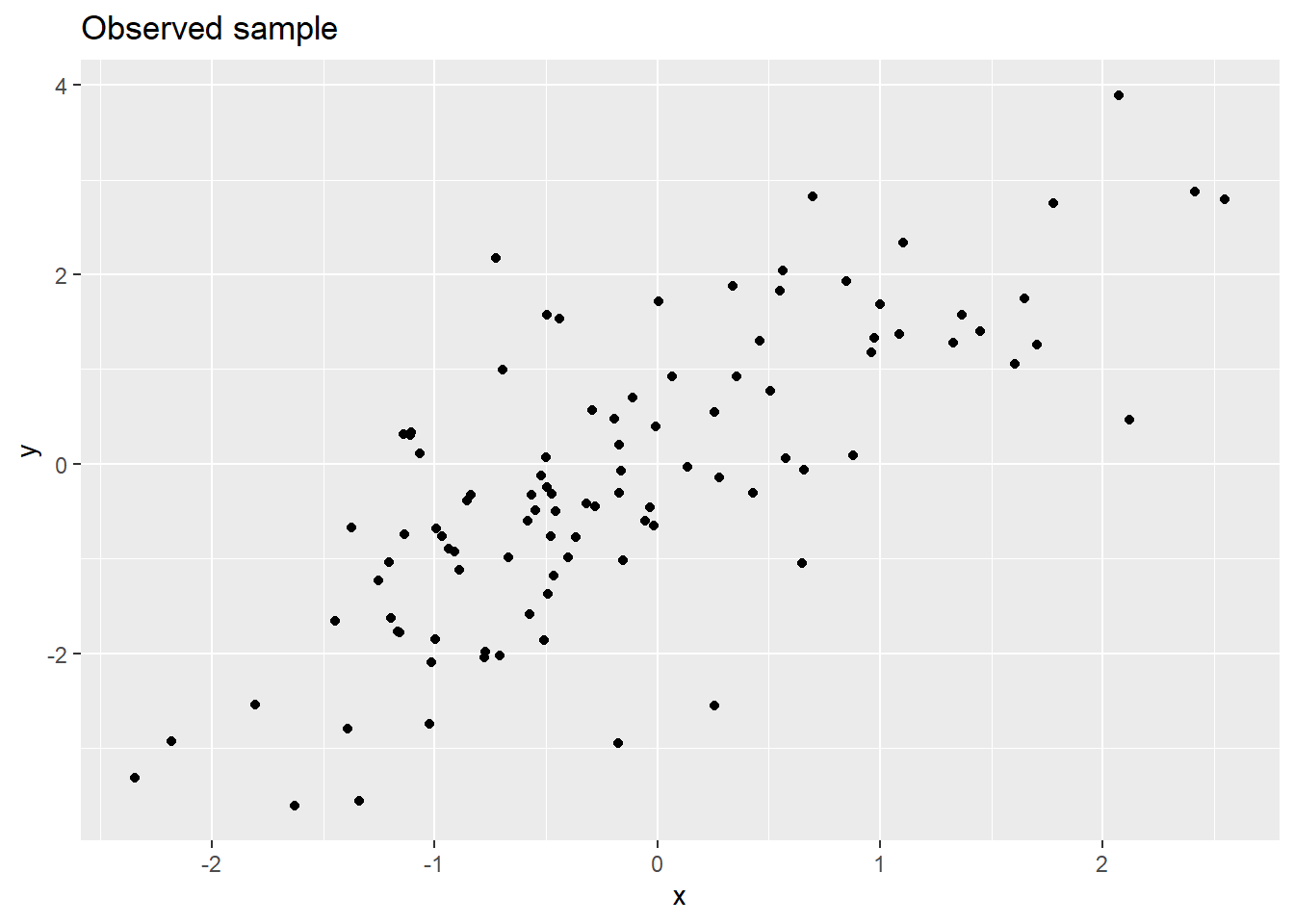

From data to log posterior

Lets say our prior for \(\theta\) is \(\mathcal{N}(0,10)\), and that we know \(\sigma=1.0\). Also, rather than working with the posterior directly, we will use the log posterior:

\[ \log p(\theta|D) = \log p(D|\theta) + \log p(\theta) - \log p(D) \] Using the log posterior enables us to ignore \(p(D)\) in inferring \(\theta\) (as it is a constant wrt to \(\theta\)) and simplifies the multiplication into addition. Also, since the observed data \(D=\{(x_1,y_1),(x_2,y_2),...,(x_N,y_N)\}\) is a set of multiple observations to calculate \(\log p(D|\theta)\) we use that each sample is considered independent and identically distributed (iid), meaning this term is calculated as:

\[\log p(D|\theta) = \sum_i \log p(D_i|\theta)\]

For a given sample of \(D=\{(x_i,y_i)\}\) pairs, we can calculate (approximate) the log posterior as:

lprior <- function(theta) dnorm(theta,0,10,log=TRUE)
llike <- function(theta,D) sum(dnorm(D$y,D$x*theta,sd=1.0,log=TRUE))
lpost_func <- function(theta,D) llike(theta,D) + lprior(theta)

thetas <- seq(-10,10,0.01)
lpost <- numeric(length=length(thetas))
for (s in 1:length(lpost)) {
  lpost[s] <- lpost_func(thetas[s],D)
}
theta_lpost <- data.table(theta=thetas,lp=lpost)

ggplot(theta_lpost,aes(x=theta,y=lp)) +
  geom_line() +
  labs(title = "Posterior log distribution",y="unnormalised density")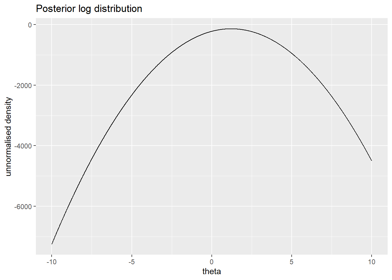

From log posterior to posterior

Rather than the log posterior we want functions of the posterior (e.g. it’s mean and quantiles). Letting \(l(\theta|D)= \log p(\theta |D)\), to calculate the posterior we normalise:

\[ p(\theta|D) = \frac{\exp [l(\theta |D)]}{Z}, Z = \int \exp [l(\theta |D)]d\theta \] Plotting the results for our sample we see the posterior is heavily centred around the true value of \(\theta=1.2\) compared to the prior \(\mathcal{N}(0,10)\), with the data massively reducing our uncertainty the value of \(\theta\).

theta_post <- data.table(theta=thetas,post=exp(lpost)/sum(exp(lpost)))
beta_post <- weighted.mean(theta_post$theta,theta_post$post)
ggplot(theta_post[post > 0],aes(x=theta,y=post)) +
  geom_line() + 
  labs(title = "Posterior distribution",y="density") +
  coord_cartesian(xlim=c(0.8,1.8))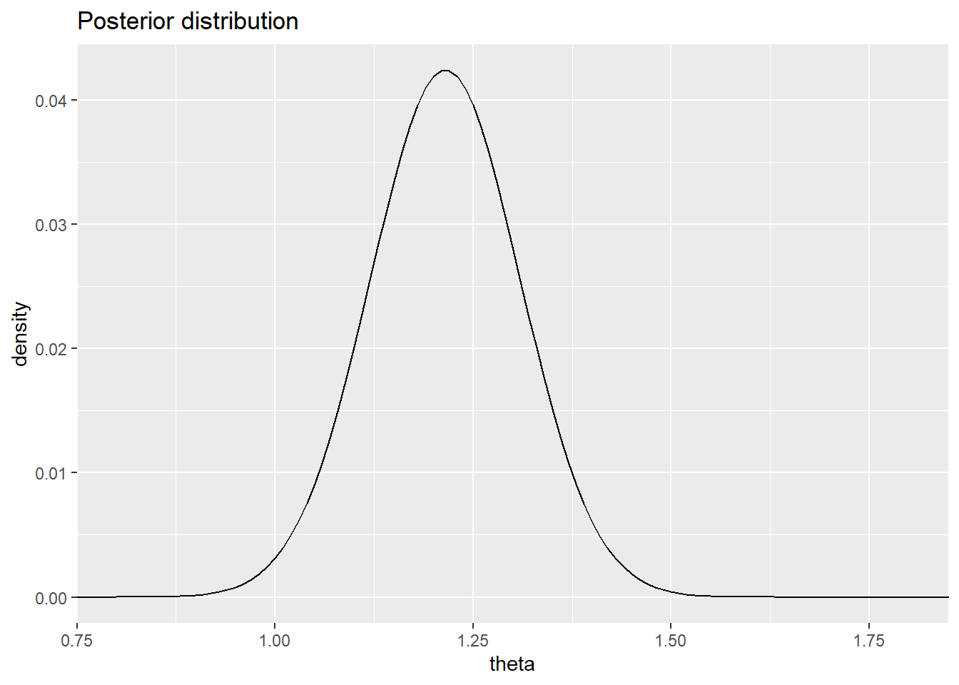

From posterior to a point estimate and credible intervals

As a point estimate (best single guess), we will use the posterior mean \(E[\theta|D]=\int\theta \cdot p(\theta |D)d \theta\). In code we can calculate this as:

theta_post[,weighted.mean(theta,post)]

[1] 1.214853

We can get 95% (credible) intervals around \(E[\theta|D]\) by finding the \(2.5^{th}\) and \(97.5^{th}\) percentiles of \(p(\theta |D)\):

theta_post[,cprob := cumsum(post)]
lower <- theta_post[cprob > 0.025,min(theta)]
upper <- theta_post[cprob <= 0.975,max(theta)]
c(lower,upper)

[1] 1.03 1.39

Next steps

This post looked at the basics of using Bayes theory for statistical inference in a semi-realistic model. A nice characteristics of Bayesian modelling is that as everything is probabilistic it is easy (theoretically) to calculate probability distributions for predictions that incorporate uncertainty from parameter estimates and the data generating process, e.g. say we observed \(x_{new}\) and want to predict the most likely range of values for \(y\). This can be done as:

\[ p(y|x_{new},D) = \int p(y|x_{new},\theta)p(\theta | D) d \theta \]

This is the posterior predictive distribution, and a topic for the next post.