Evaluating discriminatory ability of prediction models for competing risks outcomes

Background

A note on scope: this post focuses on discrimination, the ability of a model to rank subjects correctly. A model can have excellent discrimination while being miscalibrated for absolute risk, so in practice discrimination metrics should be paired with a calibration assessment (e.g. the Brier score).

AUC-ROC and the c-index

Every data scientist learns early in their statistical and machine learning studies how to evaluate binary classification models. In the case where the prediction model outputs a probability (or a score) the area under the receiver operating characteristic curve (AUC-ROC) is a common metric. The AUC-ROC can be defined in several ways. Here I use the concordance or ranking motivated definition. If \(Y \in \{0,1\}\) is our binary outcome (e.g. yes/no heart disease), \(X=x_i\) the observed prediction data (e.g. age, blood pressure, family history) for subject \(i\), \(m(\cdot)\) our model, and \(m(x_i)\) a prediction (e.g. probability of heart disease) then the AUC-ROC can be defined as:

\[ \operatorname{AUC\text{-}ROC} = \mathbb{P}\!\left( m(x_i) > m(x_j) \,\middle|\, y_i = 1, y_j = 0 \right) \]

This states the AUC-ROC for a model \(m\) is the probability \(m\) gives a higher score to a random subject with \(y=1\) compared to random subject with \(y=0\). A straightforward way to calculate this is to randomly sample \(M\) \((y_i=0,y_j=1)\) pairs and calculate the proportion of the times \(m(x_i) > m(x_j)\). This Monte-Carlo definition has some sampling error inversely proportional to \(M\) and is rarely used in practice but provides a strong intuition for the metric. The AUC-ROC is closely related to the concordance index (c-index), a metric commonly used in biostatistics. Indeed, in the binary classification case, with no need to consider the timing of the event the definitions of the AUC-ROC and c-index are equivalent. This becomes important later when they diverge in meaning!

Competing risks

Compared to the binary classification case competing risks data adds the complication of both multiple outcomes (although often there is a single “event of interest”) and a need to consider the time to the event. An example would be predicting chance of death from cardiovascular versus non-cardiovascular events. A further complication is censoring, which I will ignore for this post. Now the data has multiple mutually exclusive outcomes \(Y \in \{1,2,...\}\) and a time \(T\) at which the first outcome occurs. If we assume that \(Y=1\) is the event of interest, we have a model \(m\) that takes inputs \(X=x_i\) and time \(t\) and predicts the chance the event has occured:

\[ m(x_i,t) = \mathbb{P}\!\left(Y = 1, T \le t ,\middle|\,X = x_i\right) \]

This quantity is the cumulative incidence function (CIF) for event 1 at time \(t\), often writted as \(F_1\left(t \middle|\,X = x_i\right)\). It is the natural target for absolute risk prediction under competing risks, in contrast to alternatives such as the cause-specific hazard. The time dependent model and competing risks data structure doesn’t immediately fit into the above definition cross-sectional definition of the AUC-ROC/c-index (e.g. what to do about time and multiple events), necessitating an adaptation.

Assessing model discrimination

AUC-ROC

Accounting for time in adapting the AUC-ROC to the time-to-event setting is relatively straightforward (although see discussion of cumulative/incident distinction below). We simply introduce landmark times \(\tau\) at which we will evaluate the model based on what has happened up to the point. Slightly more complex is determining when to give the model credit for having correctly discriminated between cases (those with the event of interest) and controls (here the definition varies!). Two scenarios are possible. A model can be considered correct when it gives higher scores to subjects who experience event 1 by \(\tau\), with controls defined as everyone who is still event-free at \(\tau\) OR has experienced a competing event by \(\tau\). This leads to the following definition of time dependent AUC-ROC:

\[ \operatorname{AUC\text{-}ROC}(\tau) = \mathbb{P}\!\left( m(x_i, \tau) > m(x_j, \tau) \,\middle|\, y_i = 1,\ T_i \leq \tau,\ T_j > \tau \ \lor\ (y_j \neq 1 \land T_j \leq \tau) \right) \]

Alternatively, a model can be considered correct only when it gives higher scores to subjects who experience event 1 by \(\tau\) compared to everyone still event-free at \(\tau\):

\[ \operatorname{AUC\text{-}ROC}^*(\tau) = \mathbb{P}\!\left( m(x_i, \tau) > m(x_j, \tau) \,\middle|\, y_i = 1,\ T_i \leq \tau,\ T_j > \tau \right) \]

The difference between the two is how competing events \(Y \ne 1\) are treated. \(\operatorname{AUC\text{-}ROC}(\tau)\) places subjects with competing events into the control set and the model is penalised if it gives them a high score. \(\operatorname{AUC\text{-}ROC}^*(\tau)\) excludes them entirely, effectively treating competing events like censoring.

When the two outcomes are highly correlated (in a counterfactual sense, since we only observe one) the model would need to be good at identifying event 1 specific events compared to other events to get a high score on \(\operatorname{AUC\text{-}ROC}\), whereas \(\operatorname{AUC\text{-}ROC}^*\) might still give a high score. For instance, consider predicting death from cardiovascular events (event 1) and death from non-cardiovascular events (event 2) with simple demographic predictors such as age and gender. These outcomes are highly correlated and difficult to separate with any great strength using these predictors. However, \(\operatorname{AUC\text{-}ROC}^*(\tau)\) could still give a reasonably high score since it doesn’t ask “in those older subjects who died from cardiovascular disease, was their score higher than those who died of non-cardiovascular events”, i.e. can it separate events, but only “is the score higher in those who died from cardiovascular disease already compared to those who are still alive”.

Cumulative/Dynamic vs Incident/Dynamic

I claimed that accounting for time is straightforward, but just like the definition of a control there are several ways you can account for time the \(\operatorname{AUC\text{-}ROC}\) in time-to-event settings. Within the framework of Heagerty and Zheng (2005) the above definitions above are both cumulative/dynamic (C/D) AUC-ROCs, with a case being anyone who has had the event by \(\tau\) (cumulative), and a control is anyone still at risk at \(\tau\) (dynamic). An alternative is the incident/dynamic (I/D) AUC-ROC, where cases are subjects experiencing the event exactly at \(\tau\):

\[ \operatorname{AUC\text{-}ROC}^{I/D}(\tau) = \mathbb{P}\!\left( m(x_i, \tau) > m(x_j, \tau) \,\middle|\, y_i = 1,\ T_i = \tau,\ T_j > \tau \right) \]

C/D is the natural choice for fixed-horizon risk prediction (“5-year cardiovascular risk”). I/D is more naturally tied to the hazard, and Heagerty and Zheng (2005) show that the c-index can be written as a weighted average of \(\operatorname{AUC}^{I/D}(\tau)\) over \(\tau\). A third variant (incident/static) fixes the control set at some long-term event-free time and I won’t discuss it here.

c-index

The c-index adds an additional component to the evaluation - whether the model gives higher scores to subjects whose events happened earlier. As with the time-dependent AUC-ROC there are at least two definitions depending on who is a control, but I will simply mention the \(\operatorname{AUC\text{-}ROC}(\tau)\) style definition:

\[ C(\tau) = \mathbb{P}\!\left( m(x_i, \tau) > m(x_j, \tau) \,\middle|\, y_i = 1,\ T_i \leq \tau,\ T_j > T_i \ \lor\ (y_j \neq 1 \land T_j \leq T_i) \right) \]

Although the change can appears small and subtle they can dramatically alter the metric value. The c-index is less reported as time-varying metric you might calculate across multiple landmark times but more a single summary across all time, with \(\tau\) serving more as a upper limit. Indeed, as noted it is equal to \(\int \operatorname{AUC}^{I/D}(t) \, w(t) \, dt\).

Summary of variants

Metric	Case	Control	Competing events	R function
\(\operatorname{AUC\text{-}ROC}(\tau)\) (C/D)	\(y_i=1\), \(T_i \leq \tau\)	\(T_j > \tau\) or \(y_j \neq 1, T_j \leq \tau\)	In controls	timeROC::timeROC, riskRegression::Score
\(\operatorname{AUC\text{-}ROC}^*(\tau)\) (C/D)	\(y_i=1\), \(T_i \leq \tau\)	\(T_j > \tau\)	Excluded	timeROC::timeROC (cause-specific)
\(\operatorname{AUC\text{-}ROC}^{I/D}(\tau)\)	\(y_i=1\), \(T_i = \tau\)	\(T_j > \tau\)	(variant-dependent)	survAUC, timeROC options
\(C(\tau)\)	\(y_i=1\), \(T_i \leq \tau\)	\(T_j > T_i\) or \(y_j \neq 1, T_j \leq T_i\)	In controls	pec::cindex, riskRegression::Score

A note on censoring

I’ve ignored censoring throughout the definitions above, but in practice it is the rule rather than the exception. All the metrics above need to be estimated from data where some subjects are lost to follow-up before \(\tau\) (or before \(T_i\), for the c-index). The standard approach is inverse probability of censoring weighting (IPCW), developed for the AUC-ROC under competing risks by Blanche, Dartigues, and Jacqmin-Gadda (2013). Under the assumption that censoring is independent of the event process (conditional on covariates if needed), IPCW gives consistent estimates of the underlying probabilities. Both R functions riskRegression::Score and timeROC implement this automatically.

Example in R

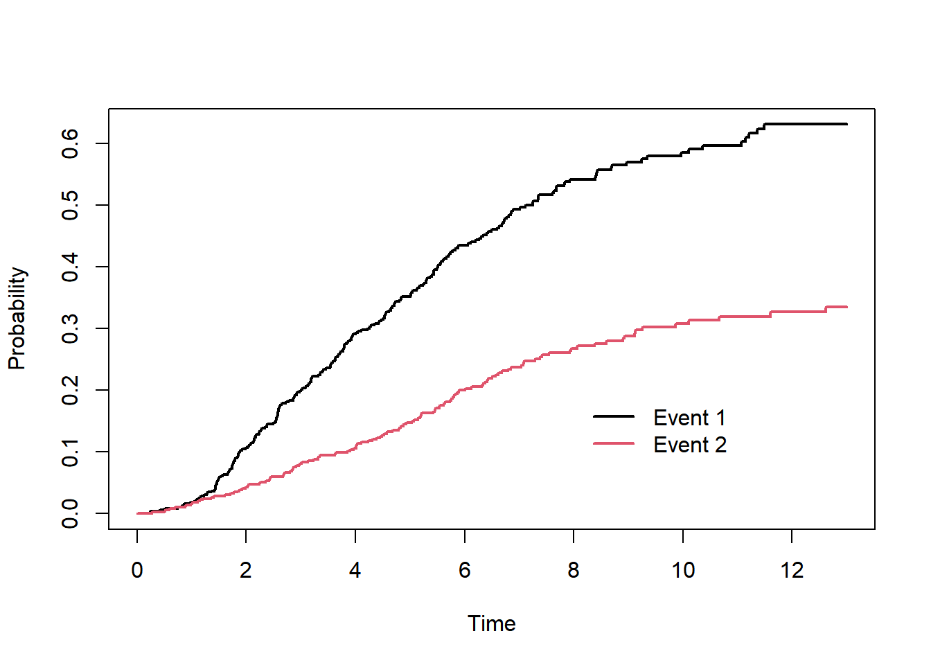
Below is a toy example comparing different R packages and their different implementations of the AUC-ROC. The graph is the cumulative incidence of the two events using the Aalen-Johansen method (a generalisation of Kaplan-Meier to multiple events).

library(survival)
library(riskRegression)
library(prodlim)
library(timeROC)
library(survAUC)

# Simulate competing risks data
set.seed(123)
df <- prodlim::SimCompRisk(500)

df$event_f <- factor(df$event, 0:2, c("censored", "Event 1", "Event 2"))

# The correct Aalen-Johansen curves
ajfit <- survfit(Surv(time, event_f) ~1, data = df)
plot(ajfit, xmax = 13, col = 1:2, lwd = 2,
     xlab = "Time", ylab = "Probability")
legend(8, .2, c("Event 1", "Event 2"), lty = 1, lwd = 2, col = 1:2, bty = 'n')

First package is riskRegression::Score, which handles AUC-ROC, Brier score, and IPCW adjustment for censoring in one call. To be honest, it is the only one I’m completely clear on how to use and what it is calculating. The other example codes are just that, generated examples.

# Fit two cause-specific Cox models combined via CSC()
fit <- CSC(Hist(time, event) ~ X1 + X2, data = df)

# --- riskRegression ---
# Evaluate at a 5-year horizon, with IPCW for censoring
sc <- Score(
  list("CSC" = fit),
  formula = Hist(time, event) ~ 1,
  data = df,
  times = 5,
  cause = 1,
  summary = "ipa",
  metrics = c("auc", "brier")
)

sc$AUC$score

Key: <model, times>
    model times       AUC         se     lower     upper
   <fctr> <num>     <num>      <num>     <num>     <num>
1:    CSC     5 0.8172512 0.02156394 0.7749866 0.8595157

sc$Brier$score

Key: <model, times>
        model times       IPA     Brier          se     lower     upper
       <fctr> <num>     <num>     <num>       <num>     <num>     <num>
1: Null model     5 0.0000000 0.2278173 0.006701120 0.2146834 0.2409513
2:        CSC     5 0.3010196 0.1592398 0.009704108 0.1402201 0.1782595

timeROC::timeROC which also which handles AUC-ROC and IPCW adjustment for censoring in one call and reports \(\operatorname{AUC\text{-}ROC}(\tau)\) and \(\operatorname{AUC\text{-}ROC}^*(\tau)\)

# --- timeROC ---
# Feed in the predicted CIF at t = 5 as the marker
risk_t5 <- as.numeric(predictRisk(fit, newdata = df, times = 5, cause = 1))

roc <- timeROC(
  T = df$time,
  delta = df$event,
  marker = risk_t5,
  cause = 1,
  weighting = "marginal",
  times = 5,
  iid = TRUE
)
# AUC_1: control = T_j > t (AUC-ROC*)
roc$AUC_1

      t=0       t=5 
       NA 0.8310065 

# AUC_2: control = T_j > t OR competing event by t (AUC-ROC)
roc$AUC_2

      t=0       t=5 
       NA 0.8172512 

The survAUC package is for standard survival outcomes, not competing risks. However it can calculate \(\operatorname{AUC\text{-}ROC}^*(\tau)\), illustrating the competing events as censoring assumption. It offers several ways to calculate the AUC-ROC and I’m not too familiar with the differences, and choose Uno et al. (2007).

# --- survAUC ---
#| label: survAUC
#| message: false
#| warning: false
#| 
# Outcome has to be a Surv() object
S <- Surv(df$time, as.numeric(df$event == 1))

# Uno's IPCW-based C/D AUC at t = 5
auc_uno <- AUC.uno(S, S, risk_t5, times = 5)
auc_uno$auc

[1] 0.8291865

For the c-index under competing risks, pec::cindex is the standard option:

library(pec)
ci <- cindex(
  list("CSC" = fit),
  formula = Hist(time, event) ~ 1,
  data = df,
  cause = 1,
  eval.times = 5
)
ci$AppCindex

$CSC
[1] 0.7742711

Which metric to use?

It is clearly use case dependent, for instance \(\operatorname{AUC\text{-}ROC}^*(\tau)\) treats competing events as censoring, which is only useful if you are happy with that assumption. Although typically you are not, since the whole point of a competing-risks framing is that those events \(Y \ne 1\) are real and informative. If you have time-varying covariates (which I didn’t cover) then it makes sense to use \(\operatorname{AUC\text{-}ROC}^{(I/D)}(\tau)\) as the cumulative versions

In many cases \(m(\cdot)\) predicts something over a fixed horizon, e.g. the probability of death from cardiovascular disease in the next 5 years. Here we really use \(m'(\cdot)\) where \(m'(x_i) = m(x_i,t=5)\), making choice of \(\tau\) for the c-index obvious. Further, \(m'\) might not even be an output from a time to event model, rather it is could be a binomial logistic regression.

It can take a while to be completely clear about package use, and exactly which metric is being output. I only felt comfortable with riskRegression::Score once I could get similar AUC-ROC and Brier scores using my own poorly implemented versions of the metrics, and have never been able to completely match the IPCW estimates, although I think I understand why…

It is important to consider measures of calibrations, for instance, when you call the R function pec::cindex you get the warning: The C-index is not proper for t-year predictions. Blanche et al. (2018), Biostatistics, 20(2): 347--357. Here they are referring to proper scoring rules. The c-index can be optimised by models that are badly miscalibrated for absolute risk, the model gets the ranking right but the probabilities wrong. This is why it should be paired with a proper scoring rule like the Brier score (or a scaled version) that rewards both discrimination and calibration.

References

Antolini, Laura, Patrizia Boracchi, and Elia Biganzoli. 2005. “A Time-Dependent Discrimination Index for Survival Data.” Statistics in Medicine 24 (24): 3927–44.

Blanche, Paul, Jean-François Dartigues, and Hélène Jacqmin-Gadda. 2013. “Estimating and Comparing Time-Dependent Areas Under Receiver Operating Characteristic Curves for Censored Event Times with Competing Risks.” Statistics in Medicine 32 (30): 5381–97.

Gerds, Thomas A, Michael W Kattan, Martin Schumacher, and Changhong Yu. 2013. “Estimating a Time-Dependent Concordance Index for Survival Prediction Models with Covariate Dependent Censoring.” Statistics in Medicine 32 (13): 2173–84.

Heagerty, Patrick J, and Yingye Zheng. 2005. “Survival Model Predictive Accuracy and ROC Curves.” Biometrics 61 (1): 92–105.

Uno, Hajime, Tianxi Cai, Lu Tian, and Lee-Jen Wei. 2007. “Evaluating Prediction Rules for t-Year Survivors with Censored Regression Models.” Journal of the American Statistical Association 102 (478): 527–37.

Wolbers, Marcel, Paul Blanche, Michael T Koller, Jacqueline CM Witteman, and Thomas A Gerds. 2014. “Concordance for Prognostic Models with Competing Risks.” Biostatistics 15 (3): 526–39.

Wolbers, Marcel, Michael T Koller, Jacqueline CM Witteman, and Ewout W Steyerberg. 2009. “Prognostic Models with Competing Risks: Methods and Application to Coronary Risk Prediction.” Epidemiology 20 (4): 555–61.