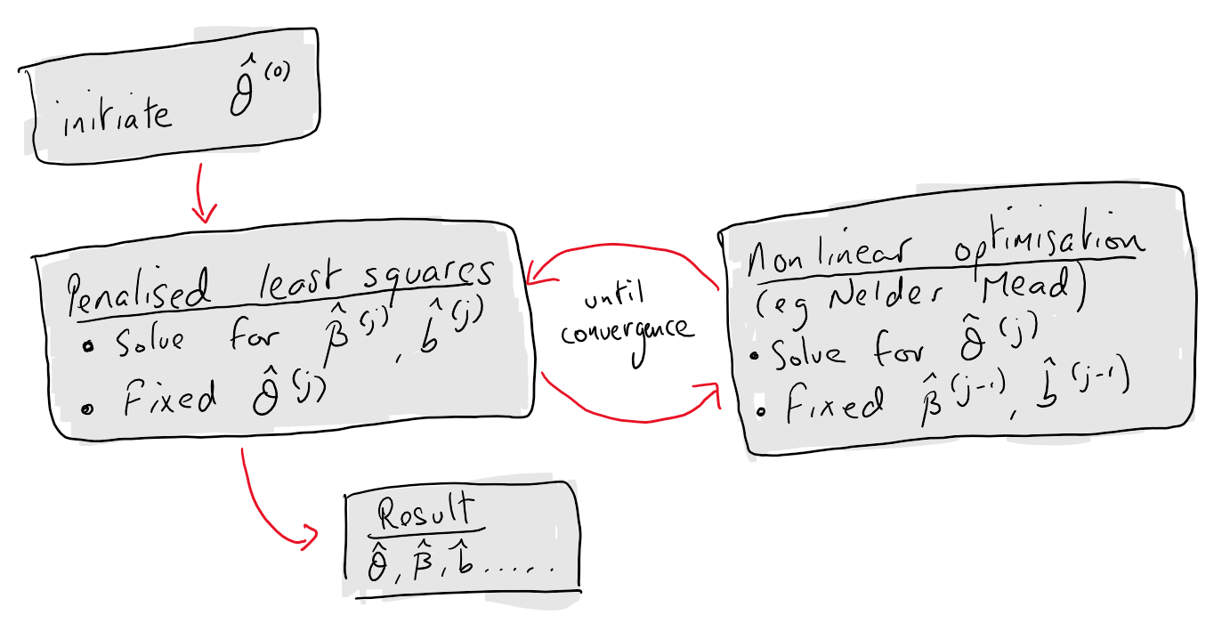
As mentioned LMMs are tricky to estimate, largely due to the presence of the unobserved random effects and additional need to decompose the outcome variance into several variance-covariance parameters. It is worth understanding the estimation process at least superficially as it can aid in debugging (commonly “why is my model taking so long to estimate!?”) and understanding warning messages when using well tested packages written by others.
Theory
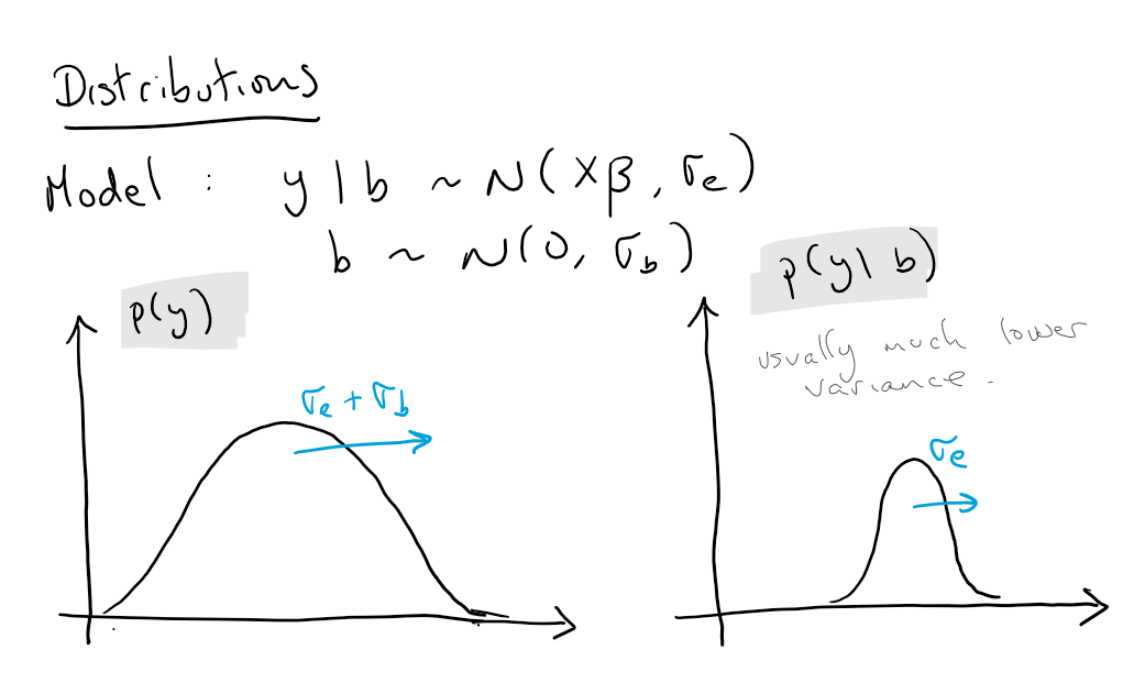
Feel free to skim this section. A common approach to estimation of LMMs is maximum likelihood estimation (MLE) or restricted MLE (REML) - but I’ll just cover MLE here. As noted in Wood (2017) estimation of \(\beta\) and \(\theta\) could be based on the marginal distribution \(p(y)\) of the outcome
\[y \sim N(X\beta,Z^t\Lambda_{\theta}Z + \Sigma_{\theta})\]
however this would involve the inversion of a \(Nn \times Nn\) matrix \(Z^t\Lambda_{\theta}Z + \Sigma_{\theta}\). As a result estimation is generally based on the the expression
\[p(y) = \int p(y,b) db = \int p(y|b)p(b) db\]
It is worth listing out some the log pdf of the distributions that are going to come up in the derivation of a the final expression. The log transform is taken to remove the exponents and convert multiplication into addition. Here and below \(c_x\) denotes a normalising constant for the distribution of \(x\).
- \(\text{log}p(y,b) = \text{log}p(y|b) + \text{log}p(b)\)
- \(\text{log}p(y|b) = c_{y|b} + \text{log}|\Sigma_{\theta}| - (y - X\beta - Z b)^t \Sigma_{\theta}^{-1} (y - X\beta - Z b)\)
- \(\text{log}p(b) = c_{b} + \text{log}|\Lambda_{\theta}| - b^t \Lambda_{\theta}^{-1} b\)
Now we are ready to derive the estimation equations. Let \(\hat{b}\) be the MLE of \(p(y,b)\). Then utilising a Taylor expansion of \(p(y,b)\) about \(\hat{b}\) on the second line below we have
\[\begin{align}
p(y) &= \int f(y,b) db = \int \text{exp}\{\text{log} p(y,b)\}db \\
&= \int \text{exp}\{\text{log} p(y,\hat{b}) + (b-\hat{b})^t \frac{\partial^2 \text{log} p(y,\hat{b})}{\partial b \partial b^t} (b-\hat{b})\}db \\
&= p(y,\hat{b}) \int \text{exp}\{-(b-\hat{b})^t (Z^t\Sigma_{\theta}^{-1} Z + \Lambda_{\theta}^{-1})(b-\hat{b})/2\}db \\
\end{align}\]
The term inside the integral can be recognised is an un-normalised Gaussian pdf with covariance \((Z^t\Sigma_{\theta}^{-1} Z + \Lambda_{\theta}^{-1})^{-1}\). The normalisation constant for this pdf would be \(\sqrt{|(Z^t\Sigma_{\theta}^{-1} Z + \Lambda_{\theta}^{-1})^{-1}| (2\pi)^{n}}\) and so, using the fact that \(|A^{-1}| = |A|^{-1}\) the result of the integral is
\[\begin{align}
p(y) &= p(y|\hat{b})p(\hat{b}) |(Z^t\Sigma_{\theta}^{-1} Z + \Lambda_{\theta}^{-1})^{-1}|^{-1/2} c_y \\
\end{align}\]
In practise we will work with the deviance (minus two times the log-likelihood), inputting our expressions for \(\text{log} p(y|b)\) and \(\text{log} p(b)\) from above gives the quantity to be minimised as
\[
d(\beta,\theta) = -2l(\beta,\theta) = (y - X\beta - Zb)^t \Sigma_{\theta}^{-1} (y - X\beta - Zb) + b^t \Lambda_{\theta}^{-1} b +
\text{log}|Z^t\Sigma_{\theta}^{-1} Z + \Lambda_{\theta}^{-1}| + c_{y|b} + c_{b} + c_y \\
\]
Computation can be based on the observation that for a fixed \(\theta\) we can get estimates of \(\beta\) and \(b\) using the first two terms
\[
d_1(\beta,\theta) = (y - X\beta - Zb)^t \Sigma_{\theta}^{-1} (y - X\beta - Zb) + b^t \Lambda_{\theta}^{-1} b
\]
Notice that the random effects (e.g. the individual intercept or feature effect) are shrinkage estimates of what we would get if we let every unit have it’s own intercept or feature effect, hence the term penalised least squares.
Then estimates of \(\theta\) can be based on the profile likelihood (deviance) \(d_p(\theta) = d(\hat{\beta},\theta)\).
Some other observations:
- Several of the terms can be interpreted as a complexity penalties on the random effects or variance-covariance parameters.
- A nicer approach is to let \(b = \Gamma_{\theta} u\) where \(u\) is a spherical normal variable (uncorrelated equal variance) and \(\Lambda_{\theta} = \Gamma_{\theta}^t\Gamma_{\theta}\), reducing the dimension of \(\theta\) by one (Bates et al, 2014).