Binary outcome misclassification

Misclassification of binary outcome data can lead to biased estimates of model coefficients when using logistic regression. In certain situations where we have information on the stucture of the misclassification problem there exist methods to estimate bias-corrected coefficients. Such methods can also be used in cases where we are unsure of the exact structure of the misclassification problem and wish to perform sensitivity analyses.

Measurement error

In a misclassified binary outcome setting, rather than observing the true outcome of interest \(Y\), we observe \(Y^*\). Our goal is to estimate the impact of covariates \(X\) on the outcome \(Y\) using logistic regression, with particular interest in the covariate coefficients \(\beta_X\):

\[P(Y=1|X=x_i) = \sigma(\beta_0 + \beta_X x_i)\]

Where \(\sigma(x) = 1/(1+e^{-x})\) is the logistic link function and we assume the covariates \(X\) are measured without error. An important consideration is whether the measurement error is nondifferential, where the mismeasured outcome is independent of the covariates given the true outcome:

\[Y^* \perp X | Y\]

Two key quantities in bias-correcting our coefficient estimates are the sensitivity and specificity of our measurement process. The sensitivity \(\text{sens} = P(Y^*=1|Y=1)\) or true positive rate quantifies the likelihood positive observations \(Y^*=1\) are in fact positive cases \(Y=1\). The specificity \(\text{spec} = P(Y^*=0|Y=0)\) or false positive rate quantifies the likelihood negative observations \(Y^*=0\) are in fact negative cases \(Y=0\).

Likelihood and estimation

For a study of size \(n\) the likelihood for our observed data is:

\[L(\beta_0,\beta_X;Y^*,X) = \prod_{i=1}^n P(Y^*=y^*_i|X=x_i)=\prod_{i=1}^n \sum_{y=0}^1 P(Y=y|X=x_i)P(Y^*=y^*_i|X=x_i,Y=y)\]

If we assume nondifferential misclassification then the second term in the likelihood can be expressed directly in terms of the sensitivity and specificity of our measurement process:

\[ \begin{split} L(\beta_0,\beta_X;Y^*,X) &= \prod_{i=1}^n \sum_{y=0}^1 P(Y=y|X=x_i)P(Y^*=y^*_i|X=x_i,Y=y) \\ &= \prod_{i=1}^n \sum_{y=0}^1 P(Y=y|X=x_i) P(Y^*=y^*_i|Y=y) \\ &= \prod_{i=1}^n P(Y=0|X=x_i) P(Y^*=y^*_i|Y=0) + P(Y=1|X=x_i) P(Y^*=y^*_i|Y=1) \\ &= \begin{split} \prod_{i=1}^n [P(Y=0|X=x_i) P(Y^*=1|Y=0) + P(Y=1|X=x_i) P(Y^*=1|Y=1)]^{y_i} \times \\ [P(Y=0|X=x_i) P(Y^*=0|Y=0) + P(Y=1|X=x_i) P(Y^*=0|Y=1)]^{1-y^*_i} \end{split} \\ &= \begin{split} \prod_{i=1}^n [P(Y=0|X=x_i) (1-\text{spec}) + P(Y=1|X=x_i) \text{sens}]^{y^*_i} \times \\ [P(Y=0|X=x_i) \text{spec} + P(Y=1|X=x_i) (1-\text{sens})]^{1-y^*_i} \end{split} \\ \end{split} \]

Where the second line uses the nondifferential error. For optimisation purposes we often target minimising the negative log-likelihood:

\[ l(\beta_0,\beta_X;Y^*,X) = \begin{split} \sum_{i=1}^n y^*_i \text{log}[(1-\sigma(\beta_0 + \beta_X x_i)) (1-\text{spec}) + \sigma(\beta_0 + \beta_X x_i) \text{sens}] + \\ (1-y^*_i) \text{log}[(1-\sigma(\beta_0 + \beta_X x_i)) \text{spec} + \sigma(\beta_0 + \beta_X x_i) (1-\text{sens})] \end{split} \]

Notice how there is nothing in this final form of the likelihood that cannot be replaced by the observed data \((Y^*,X)\), or the known (or assumed) sensitivity and specificity values. This can now be directly optimised using general purpose optimisation routines in R (e.g. stats::optim), python (e.g. scipy.optimize) etc. See 5.4.4 of Shaw et al. (2020) for a list of papers that developed this methodology.

Bias corrected model fitting functions

The code below uses the above results to adjust the logistic regression fitting estimation process to account for the sensitivity and specificity of the measurement process.

logistic <- function(X,betas) {
    1 / (1 + exp(- (X %*% betas)))
}

nLL_mc <- function(betas,X,y,sens,spec) {
  n <- nrow(X)
  pY <- logistic(X,betas)
  t1 <- -y*log(sens*pY + (1-spec)*(1-pY))
  t2 <- -(1-y)*log((1-sens)*pY + spec*(1-pY))
  sum(t1 + t2)  
}

missclass_glm <- function(formula,sens,spec,data) {

  # initial fit ignoring missclassification
  b0 <- coef(glm(formula,data=data,family = binomial()))
  
  # fit accounting for sens and spec
  y <- model.response(model.frame(formula,data))
  X <- model.matrix(formula,data)
  res <- optim(b0,nLL_mc,X=X,y=y,sens=sens,spec=spec,hessian=TRUE)
  coef <- res$par
  std_err <- sqrt(diag(solve(res$hessian)))
  z <- coef / std_err
  p_value <- (1 - pnorm(abs(z))) * 2
  
  # output 
  list(unadjusted = b0,
       adjusted = data.table(var = names(coef),
                             coef = coef,
                             std_err = std_err,
                             p_value = p_value,
                             lower = coef - 1.96*std_err,
                             upper = coef + 1.96*std_err))
}

Simulation studies

A question for any method is how well does it work? Below we look at a few different scenarios and compare how the coefficients estimated from the bias-adjusted method compare to those estimates naively using standard logistic regression.

Data generating process

The simulated data contains five variables, three binary (A1, A2 and A3) and two continuous (X1 and X2), with A1 and X2 being the “most important” (the largest coefficients). There are no interactions and the connection between the probabilistic outcome and covariates is a straightforward logistic link.

fake_data <- function(sens,spec,betas,n=1000) {
  # data generation
  ## categorical variables
  A1 <- rbinom(n,1,0.3)
  A2 <- rbinom(n,1,0.7)
  A3 <- rbinom(n,1,0.2)
  ## continuous variables
  X1 <- rnorm(n)
  X2 <- rnorm(n)

  X <- cbind(rep(1,n),A1,A2,A3,X1,X2)
  pY <- logistic(X,betas)
  
  # flip some outcome values
  pYs <- pY*sens + (1 - pY)*(1-spec)
  Ys <- fifelse(pYs > runif(n),1,0)

  data.table(Ys = Ys, A1 = A1, A2 = A2, A3 = A3, X1 = X1, X2 = X2)
}

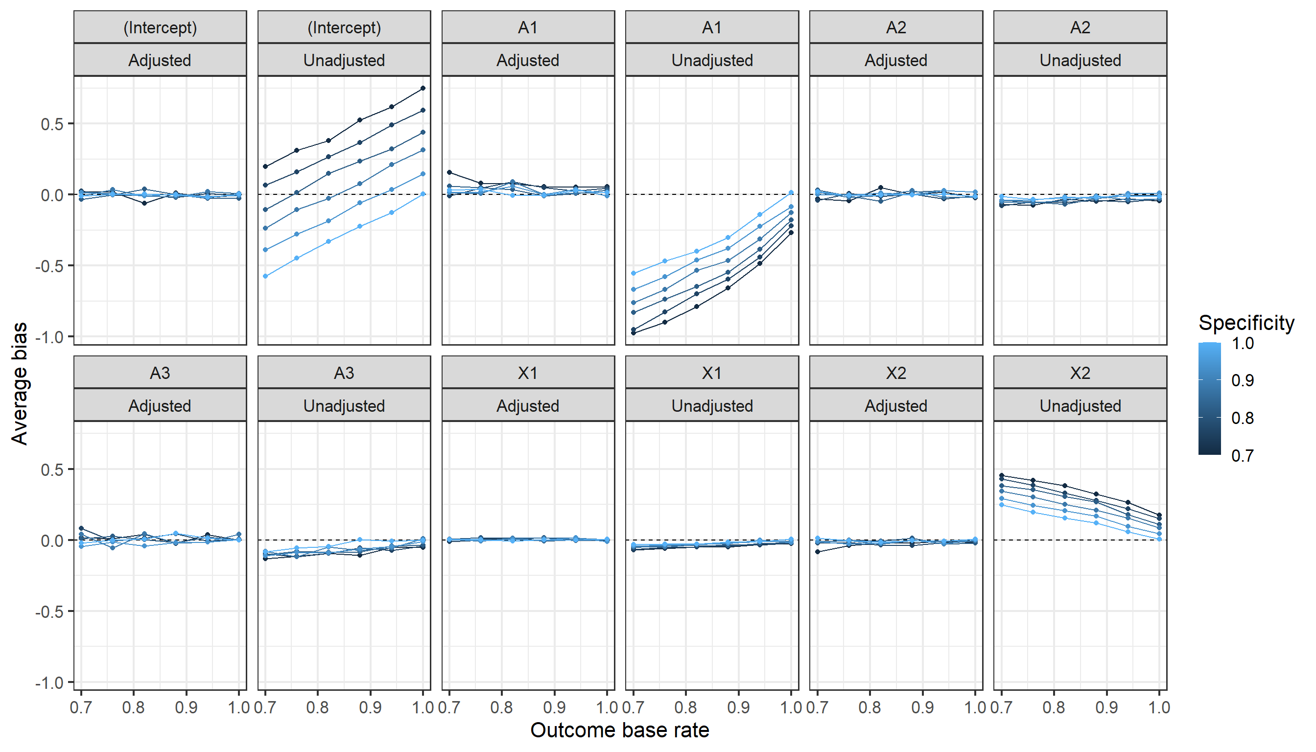
Simulation study 1: Vary sensitivity and specificity

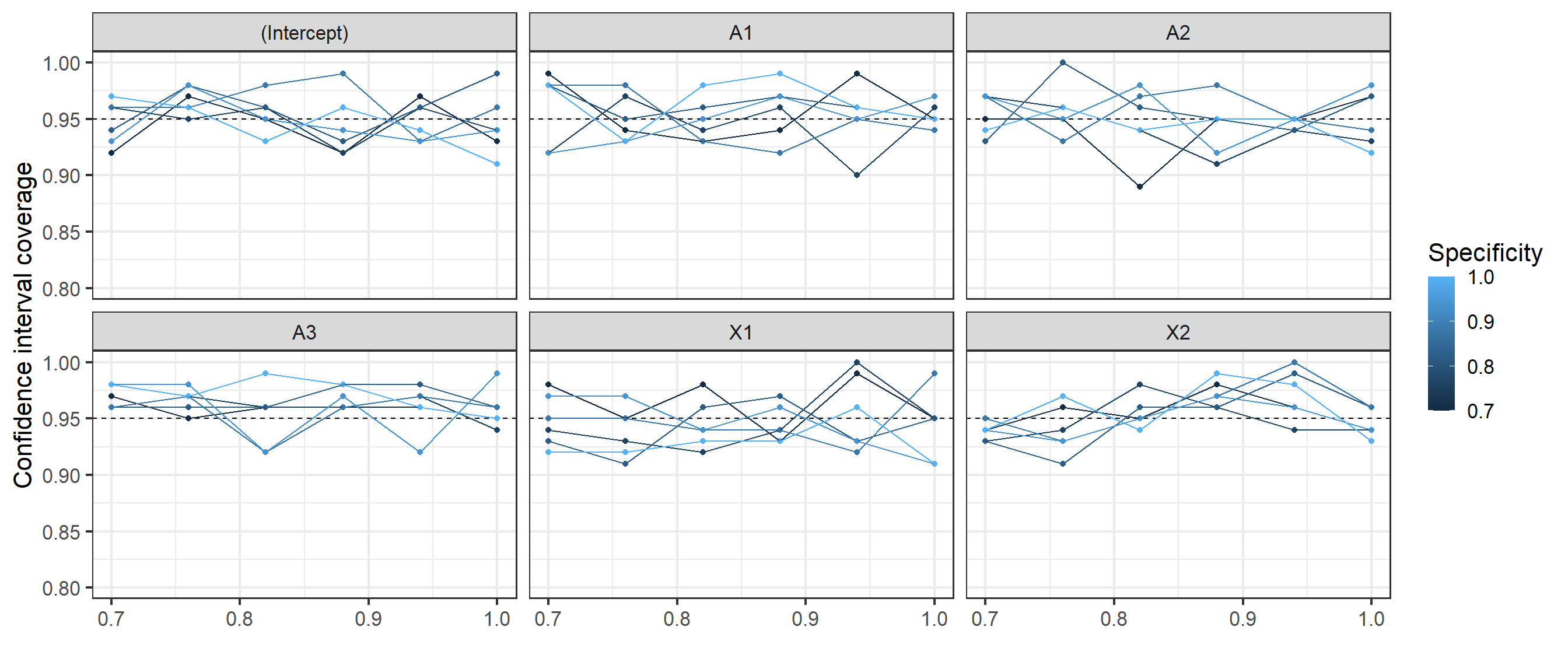
Below we vary the sensitivity and specificity of the outcome measurement process assessing the impact of this on the average bias \(B_M=\frac{1}{M}\sum_m (\hat{\beta}_m-\beta)\) across \(m=1,..,M\) simulations of the unadjusted logistic regression coefficients, and the degree to which the bias-correction estimation process accounts for any bias. We also assess the coverage of the 95% confidence intervals (Wald approximate) \(C_M=\frac{1}{M}\sum_m I_{\beta \in (\hat{\beta}_{m,\text{95% lower}},\hat{\beta}_{m,\text{95% upper}})}\) around the bias-adjusted coefficients.

M <- 100
sens <- seq(0.7,1.0,length.out=6)
spec <- seq(0.7,1.0,length.out=6)
betas <- c(-0.3,1.5,0.1,0.2,0.1,-0.7)
bias_vary_me <- vector(mode="list",length=length(sens)*length(spec))
coverage_vary_me <- vector(mode="list",length=length(sens)*length(spec))

ij <- 1
for (i in 1:length(sens)) {
    for (j in 1:length(spec)) {
        bias_orig <- vector(mode="list",length=M)
        bias_adjust <- vector(mode="list",length=M)
        coverage_adjust <- vector(mode="list",length=M)
        for (m in 1:M) {
            dt <- fake_data(betas = betas, sens = sens[i], spec = spec[j])
            models <- missclass_glm(Ys ~ A1 + A2 + A3 + X1 + X2,sens[i],spec = spec[j],dt)
            bias_orig[[m]] <- models$unadjusted - betas
            bias_adjust[[m]] <- models$adjusted$coef - betas
            names(bias_adjust[[m]]) <- models$adjusted$var
            coverage_adjust[[m]] <- fifelse(models$adjusted$lower <= betas & 
                                            models$adjusted$upper >= betas,1,0)
        }
        bias_orig <- as.data.table(do.call(rbind,bias_orig))
        bias_adjust <- as.data.table(do.call(rbind,bias_adjust))
        bias_orig[,method := "unadjusted"]
        bias_adjust[,method := "adjusted"]
        bias_ <- rbind(bias_orig,bias_adjust)
        bias_[,sens := sens[i]]
        bias_[,spec := spec[j]]
        bias_vary_me[[ij]] <- bias_

        coverage_ <- as.data.table(do.call(rbind,coverage_adjust))
        names(coverage_) <- models$adjusted$var
        coverage_ <- coverage_[,lapply(.SD,mean)]
        coverage_[,sens := sens[i]]
        coverage_[,spec := spec[j]]
        coverage_vary_me[[ij]] <- coverage_

        ij <- ij + 1
    }
}
bias_vary_me <- rbindlist(bias_vary_me)

Coefficient bias

As shown below the bias-adjusted coefficients perform far better than the unadjusted coefficients in capturing the true values of the data generating process (model coefficients).

cols <- c("(Intercept)","A1","A2","A3","X1","X2")
tab <- bias_vary_me[,lapply(.SD, mean),by=.(method,sens,spec),.SDcols=cols]
tab1 <- melt(tab,id.vars  = 1:3)
tab1[,Method := fifelse(method == "unadjusted","Unadjusted","Adjusted")]
ggplot(tab1,aes(x=sens,y=value,col=spec,group=spec)) + 
    geom_hline(yintercept = 0.0,linetype = 2) +
    geom_line() + 
    geom_point() +
    facet_wrap(~variable*Method,ncol=6) +
    labs(x = "Outcome base rate",y="Average bias") +
    scale_color_continuous(name="Specificity") +
    theme_bw(base_size=16) 

Coefficient 95% confidence interval coverage

The coverage of these lare sample confidence intervals appears reasonably close to 95% given the low number of simulation repetitions \(M=100\) and sample size \(n=1000\).

tab <- rbindlist(coverage_vary_me)
tab1 <- melt(tab,id.vars  = 7:8)
ggplot(tab1,aes(x=sens,y=value,col=spec,group=spec)) + 
    geom_hline(yintercept = 0.95,linetype = 2) +
    geom_point() +
    geom_line() +
    facet_wrap(~variable) +
    coord_cartesian(ylim = c(0.8,1.0)) +
    labs(x = "",y="Confidence interval coverage") +
    scale_color_continuous(name="Specificity") +
    theme_bw(base_size=16) 

Simulation study 2: Vary outcome base rate

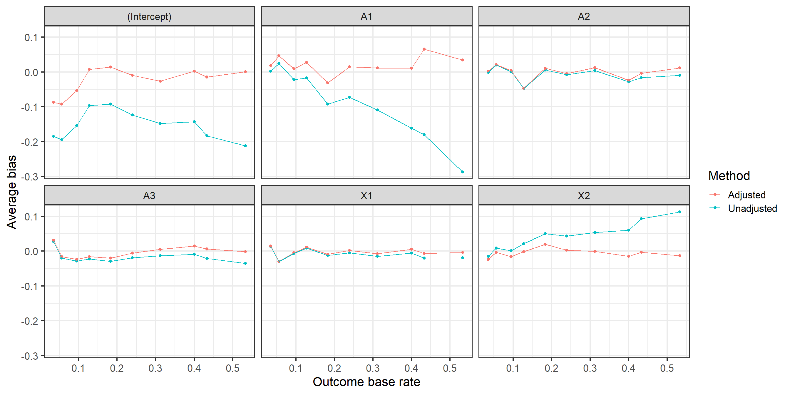
Below we assess the extent to which the degree of bias varies by the outcome base rate. We see that the degree of bias, and importance of using bias-correction matters more when the \(Y=1\) is more likely for the current simulation setup.

M <- 100
betas <- c(NA,1.5,0.1,0.2,0.1,-0.7)
b0 <- seq(-4,0,length.out = 10)
res_vary_base <- vector(mode="list",length=length(b0))
for (i in 1:length(b0)) {
    betas[1] <- b0[i]
    res_orig <- vector(mode="list",length=M)
    res_adjust <- vector(mode="list",length=M)
    y_rate <- vector(mode="numeric",length=M)
    for (m in 1:M) {
        dt <- fake_data(betas = betas, sens = 0.9, spec = 1.0)
        models <- missclass_glm(Ys ~ A1 + A2 + A3 + X1 + X2,0.9,1.0,dt)
        res_orig[[m]] <- models$unadjusted - betas
        res_adjust[[m]] <- models$adjusted$coef - betas
        names(res_adjust[[m]]) <- models$adjusted$var
        y_rate <- mean(dt$Ys)
    }
    res_orig <- as.data.table(do.call(rbind,res_orig))
    res_adjust <- as.data.table(do.call(rbind,res_adjust))
    res_orig[,method := "unadjusted"]
    res_adjust[,method := "adjusted"]
    res <- rbind(res_orig,res_adjust)
    res[,y_rate := mean(y_rate)]
    res_vary_base[[i]] <- res
}
res_vary_base <- rbindlist(res_vary_base)

cols <- c("(Intercept)","A1","A2","A3","X1","X2")
tab <- res_vary_base[,lapply(.SD, mean),by=.(method,y_rate),.SDcols=cols]
tab1 <- melt(tab,id.vars  = 1:2)
ggplot(tab1,aes(x=y_rate,y=value,col=method,group=method)) + 
    geom_hline(yintercept = 0.0,linetype = 2) +
    geom_point() + 
    geom_line() +
    facet_wrap(~variable) +
    labs(x = "Outcome base rate",y="Average bias") +
    scale_color_discrete(name="Method",labels=c("Adjusted","Unadjusted")) +
    theme_bw(base_size=16)

Conclusion

In this situation with nondifferential misclassification error and knowledge of the sensitivity and specificity of the measurement process the outlined method works well, demonstrating a reduction in coefficient bias that varies from small to considerable depending on aspects of the data generation process (outcome base rate) and degree of mismeasurement.

References

Shaw, Pamela A, Paul Gustafson, Raymond J Carroll, Veronika Deffner, Kevin W Dodd, Ruth H Keogh, Victor Kipnis, et al. 2020. “STRATOS Guidance Document on Measurement Error and Misclassification of Variables in Observational Epidemiology: Part 2—More Complex Methods of Adjustment and Advanced Topics.” Statistics in Medicine 39 (16): 2232–63.