Missing data and directed acyclic graphs

Missingness graphs

In many data science applications it is quite common for there to be a need to account for missing data. Missingness graphs (or m-graphs) extend traditional causal graphs by making explicit the presence of missing variables (Mohan and Pearl 2021). Let \(G(\textbf{V}, E)\) be a causal directed acyclic graph (DAG) where \(\textbf{V}\) is the set of nodes (variables) and \(E\) is the set of edges (causal relationships). The nodes are partitioned into five categories:

\[\textbf{V} = V_o \cup V_m \cup U \cup V^* \cup R\]

where \(V_o\) is the set of fully observed variables, and \(V_m\) is the set of partially observed variables. Associated with every partially observed variable are the proxy variables that is actually observed \(V^*_i\) and \(R_{v_i}\) a binary variable which represents the status of the causal mechanism responsible for the missingness of \(V^*_i\). These are related as:

\[v_i^* = f(r_{v_i},v_i) = \begin{cases} v_i, & \text{if $r_{v_i} = 0$} \\ m, & \text{if $r_{v_i} = 1$} \end{cases}\]

This simply links that the missingness indicator \(r\_{v_i}\) is one we don’t observe the variable (duh), a key question will be whether we can reasonably determine why \(r_{v_i}=1\) using the observed data. \(V^∗\) is the set of all proxy variables and \(R\) is the set of all causal mechanisms that are responsible for missingness. \(U\) is the set of unobserved nodes, also called latent variables. These sets of variables can be grouped into two to define the missing data distribution, \(P(V^∗,V_o, R)\) and the underlying distribution \(P(V_o,V_m, R)\).

Recoverability

When we have missing data we need a way to determine whether our desired parameter (statistical model, causal effect etc) is recoverable. Recoverability is defined as whether any method exists that produces a consistent estimate of a desired parameter and, if so, how.

Examples

Our target quantity is a prediction of the number of usable cleavage stage (day 3) embryos \(C\) a woman is likely to get from IVF given her age \(A\) and the number of fertilised oocytes (zygotes / day 1 embryos) \(Z\). However, our data source only records whether our embryos reached cleavage stage if they are transferred to the woman prior to blastocyst stage (day 5), with \(B\) the number of blastocysts. So we only observed \(B\) or \(C\). We’ll consider a few m-DAGs for this problem, with \(U\) an unmeasured variable representing prognosis (aka degree of infertility or oocyte/embryo quality).

1. Recoverable (missing at random)

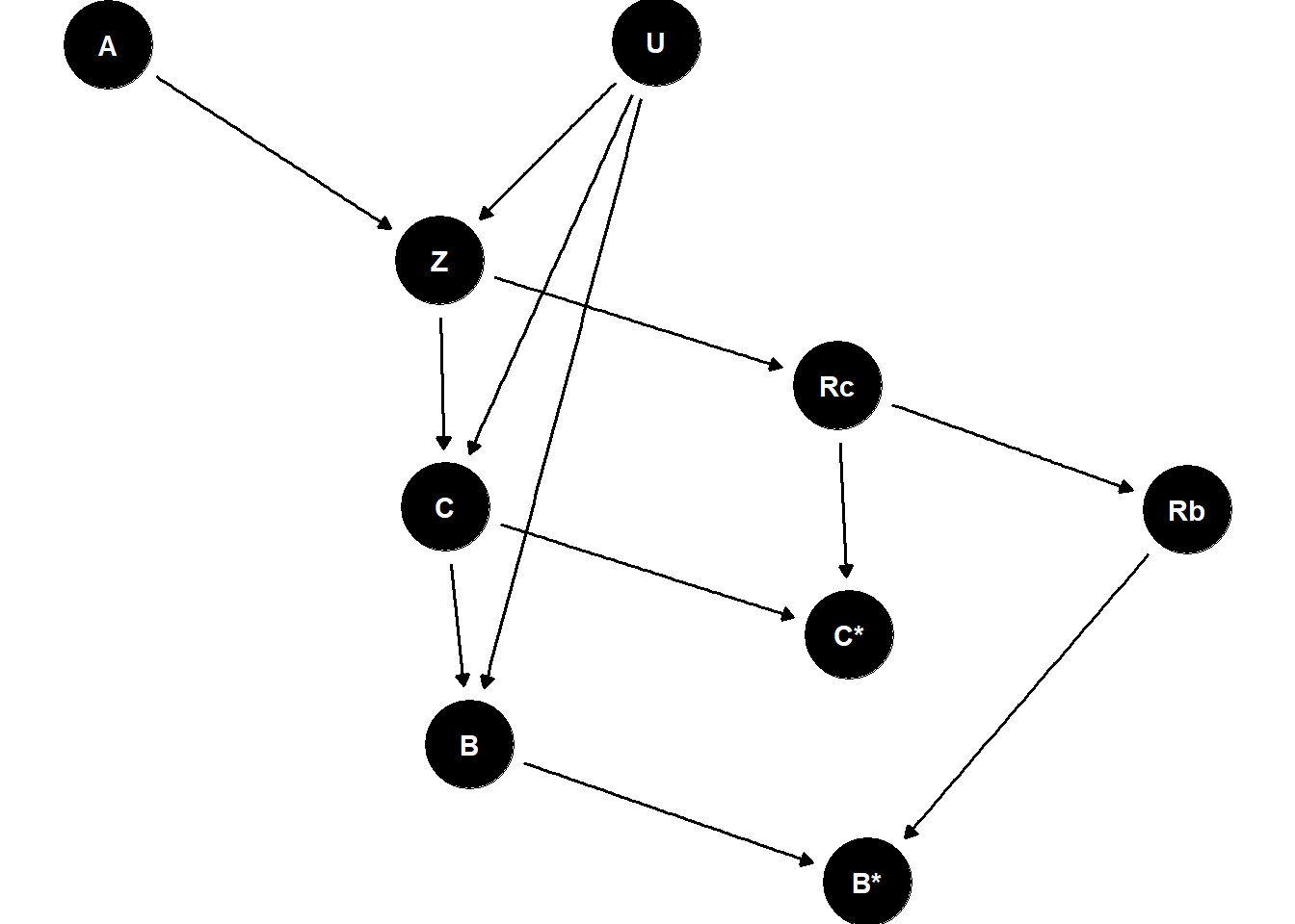
In this first m-DAG, the decision (missingness mechanism \(R_c\)) around whether to transfer at cleavage or blastocyst stage is taken based on the number of fertilised oocytes \(Z\).

dag <- dagitty('dag {
    bb="0,0,1,1"
    "B*" [pos="0.381,0.493"]
    "C*" [pos="0.378,0.416"]
    A [pos="0.255,0.232"]
    B [pos="0.315,0.450"]
    C [pos="0.311,0.376"]
    Rb [pos="0.434,0.377"]
    Rc [pos="0.376,0.338"]
    U [pos="0.346,0.231"]
    Z [pos="0.310,0.299"]
    A -> Z
    B -> "B*"
    C -> B
    C -> "C*"
    Rb -> "B*"
    Rc -> "C*"
    Rc -> Rb
    U -> Z
    U -> C
    U -> B
    Z -> C
    Z -> Rc
}')
ggdag(dag) + 
    scale_y_reverse() + 
    theme_void(base_size = 22)

f_n_zy <- function(age, prog) {
    stopifnot(length(age) == length(prog))
    n <- length(age)
    n_zy <- (age == "<35" & prog == "good") * rpois(n,6) +
    (age == "<35" & prog == "bad") * rpois(n,4) +
    (age == "≥35" & prog == "good") * rpois(n,5) +
    (age == "≥35" & prog == "bad") * rpois(n,3) + 1
    n_zy
}
f_n_cl <- function(n_zy, prog) {
    stopifnot(length(n_zy) == length(prog))
    n <- length(n_zy)
    n_cl <- (prog == "good") * rbinom(n, size = n_zy, prob = 0.7) +
    (prog == "bad") * rbinom(n, size = n_zy, prob = 0.7)
    n_cl
}
f_n_bl <- function(n_cl, prog) {
    stopifnot(length(n_cl) == length(prog))
    n <- length(n_cl)
    n_bl <- (prog == "good") * rbinom(n, size = n_cl, prob = 0.7) +
    (prog == "bad") * rbinom(n, size = n_cl, prob = 0.7)
    n_bl
}
gen_data <- function(n,f_p_bl) {
    age <- sample(c("<35","≥35"),n,prob = c(0.4,0.6),replace = TRUE)
    prog <- sample(c("good","bad"),n,prob = c(0.3,0.7),replace = TRUE)
    n_zy <- f_n_zy(age,prog)
    n_cl <- f_n_cl(n_zy, prog)
    n_bl <- f_n_bl(n_cl, prog)
    p_bl <- f_p_bl(age, n_zy, n_cl)
    bl <- runif(n) < p_bl
    data.table(age,prog,n_zy,n_cl,n_bl,p_bl,bl)
}
make_observed <- function(df) {
    df1 <- copy(df)
    df1[bl == TRUE,n_cl := NA]
    df1[bl == FALSE,n_bl := NA]
    df1[,p_bl := NULL]
    df1[,prog := NULL]
    df1
}

Based on this, conditioning on \(Z\) d-separates \(R_c\) and \(C\), \(C \perp R_c | Z\), so we can use the available data:

\[ \begin{split} P(C|A=a,Z=z) &= P(C|A=a,Z=z,R_c=0) \\ &= P(C^*|A=a,Z=z,R_c=0) \end{split} \]

If we only wanted to predict based on female age, we can also do so by summing over the distribution of \(Z\):

\[ \begin{split} P(C|A=a) &= \sum_z P(C|A=a,Z=z) P(Z=z|A=a) \\ &= \sum_z P(C|A=a,Z=z,R_c=0) P(Z=z|A=a) \\ &= \sum_z P(C^*|A=a,Z=z,R_c=0) P(Z=z|A=a) \\ \end{split} \]

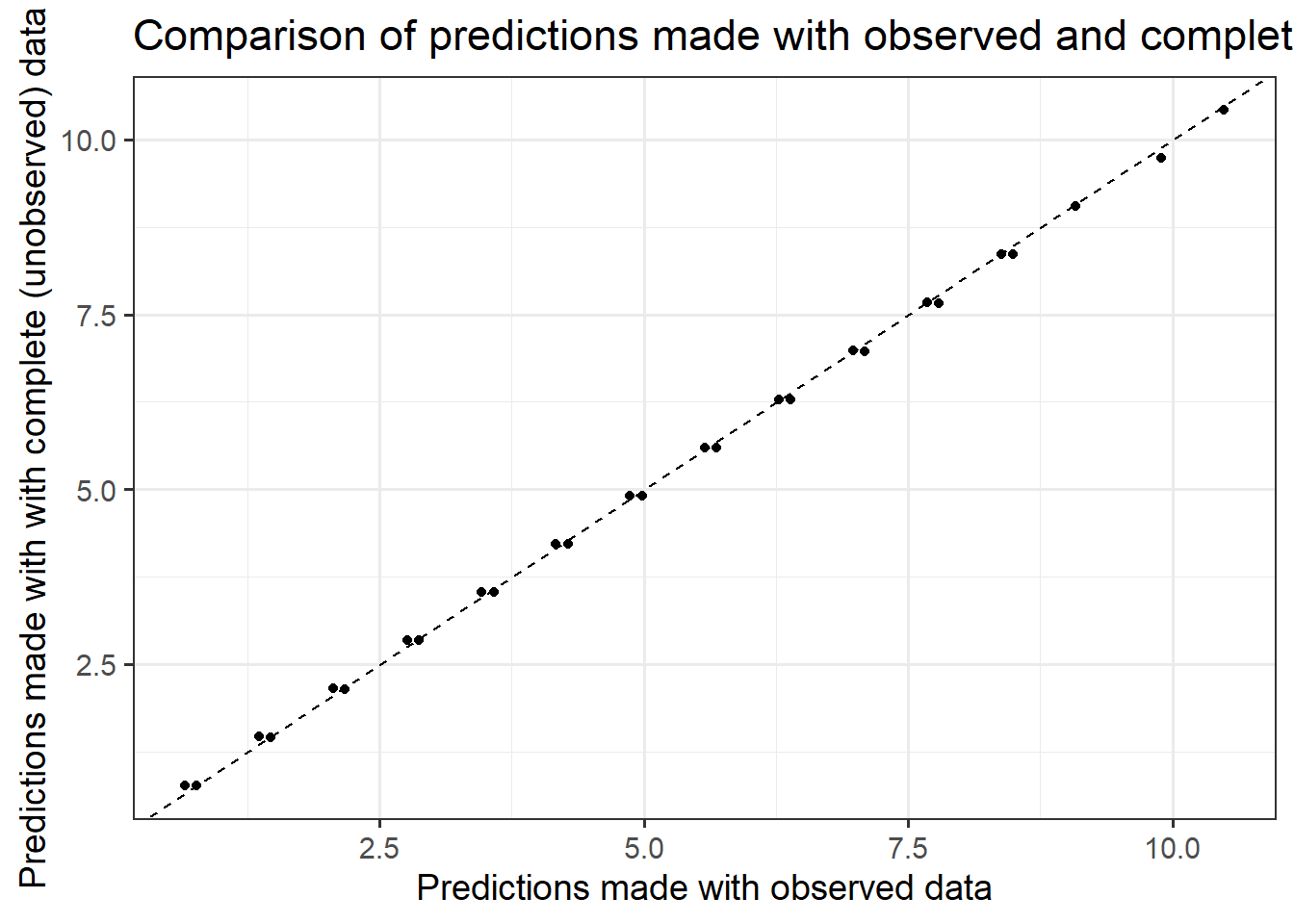
As shown below, there is no difference between models fit on the observed data (with missingness) and models fit on a theoretically complete (no missingness) dataset.

f_p_bl <- function(age, n_zy, n_cl) {
    p_bl <- fifelse(n_zy >= 4, 0.8, 0.2)
    p_bl
}
df <- gen_data(1000,f_p_bl)
df1 <- make_observed(df)
miss_cl <- lm(n_cl ~ n_zy + age, data = df1)
true_cl <- lm(n_cl ~ n_zy + age, data = df)


miss_pred = predict(miss_cl,newdata=df1)
true_pred = predict(true_cl,newdata=df1)

res_df = data.table(miss_pred, true_pred)

ggplot(res_df,aes(x = miss_pred,y=true_pred)) + 
    geom_point() +
    labs(x= "Predictions made with observed data",
         y = "Predictions made with with complete (unobserved) data",
    title = "Comparison of predictions made with observed and complete data") +
    geom_abline(intercept=0,slope=1,linetype=2)+
  theme_bw(base_size=14)

2. Recoverable (missing at random)

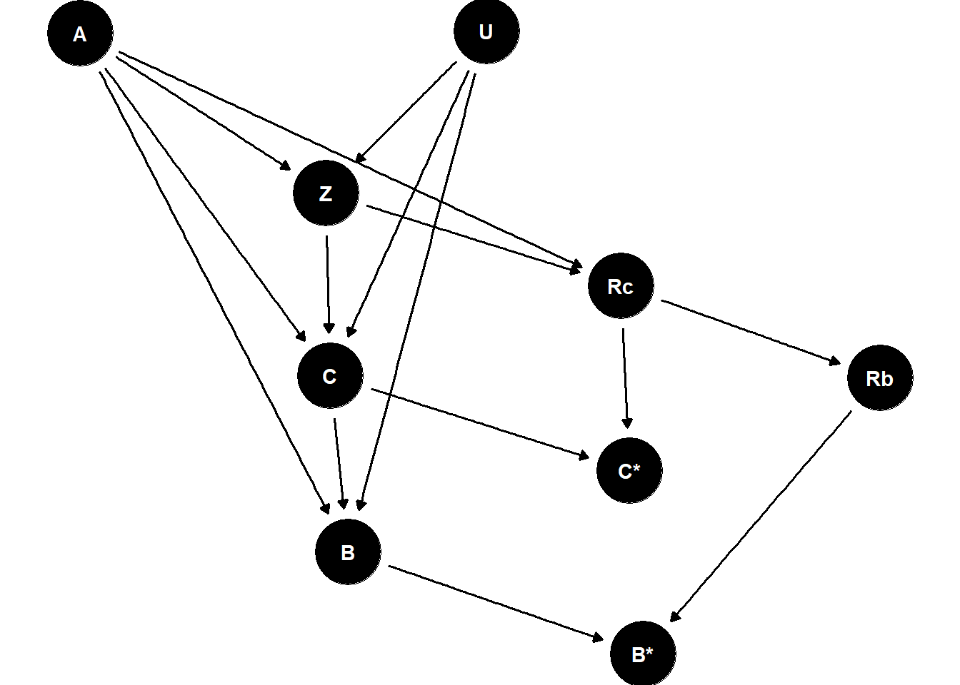
This second example expands the factors that determine the number of cleavage and blastocyst stage embryos to include female age, and the unmeasured prognosis variable. Further, female age is also used to determine whether to transfer cleavage or blastocyst stage embryos. Despite the increased complexity, things are pretty much the same, to d-separate \(C\) and \(R_c\) we need to condition on \(A\) and \(Z\) making \(P(C|A,Z)\) recoverable.

dag <- dagitty('dag {
    bb="0,0,1,1"
    "B*" [pos="0.381,0.493"]
    "C*" [pos="0.378,0.416"]
    A [pos="0.255,0.232"]
    B [pos="0.315,0.450"]
    C [pos="0.311,0.376"]
    Rb [pos="0.434,0.377"]
    Rc [pos="0.376,0.338"]
    U [pos="0.346,0.231"]
    Z [pos="0.310,0.299"]
    A -> Z
    B -> "B*"
    C -> B
    C -> "C*"
    Rb -> "B*"
    Rc -> "C*"
    Rc -> Rb
    U -> Z
    Z -> C
    Z -> Rc
    A -> C
    A -> B
    A -> Rc
    U -> C
    U -> B
}')
ggdag(dag) + 
    scale_y_reverse() + 
    theme_void(base_size = 22)

3. Missing not at random (non-recoverable)

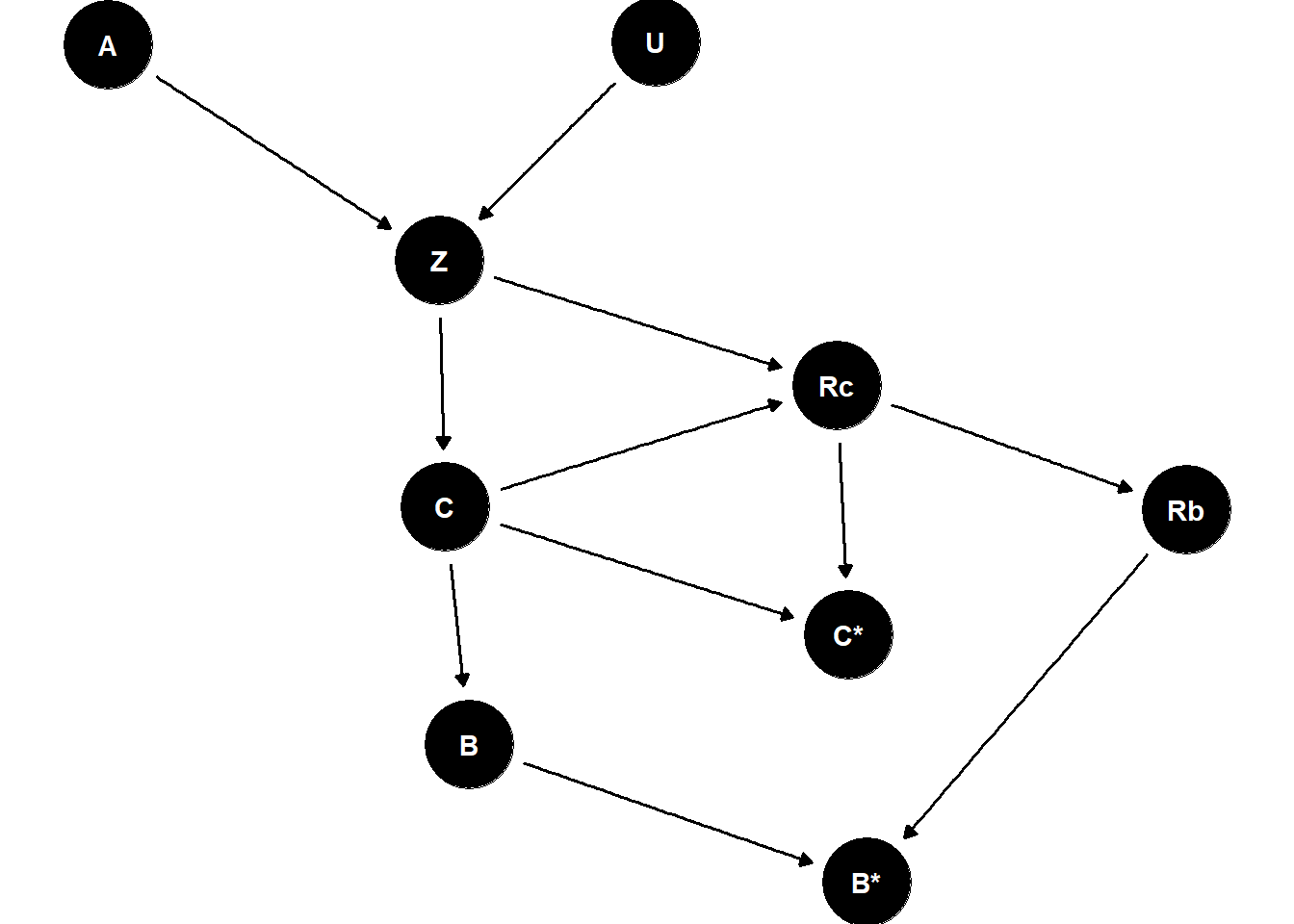
In this final example we consider a case where \(P(C|A,Z)\) is non-recoverable. The mechanism for this is vary simple, \(C\) causes its own missingness. In this IVF example this could occur if the decision to transfer at cleavage or blastocyst stage is taken based on the number of embryos that reach cleavage stage, e.g. too few have survived to cleavage then transfer (or freeze) now vs. good survival rate then continue culture to blastocyst. In the m-graph below there is no way to block the path between \(C\) and \(R_c\). This is an example of a “missing not at random” (MNAR) problem.

dag <- dagitty('dag {
    bb="0,0,1,1"
    "B*" [pos="0.381,0.493"]
    "C*" [pos="0.378,0.416"]
    A [pos="0.255,0.232"]
    B [pos="0.315,0.450"]
    C [pos="0.311,0.376"]
    Rb [pos="0.434,0.377"]
    Rc [pos="0.376,0.338"]
    U [pos="0.346,0.231"]
    Z [pos="0.310,0.299"]
    A -> Z
    B -> "B*"
    C -> B
    C -> "C*"
    Rb -> "B*"
    Rc -> "C*"
    Rc -> Rb
    U -> Z
    Z -> C
    Z -> Rc
    C -> Rc
}')
ggdag(dag) + 
    scale_y_reverse() + 
    theme_void(base_size = 22)

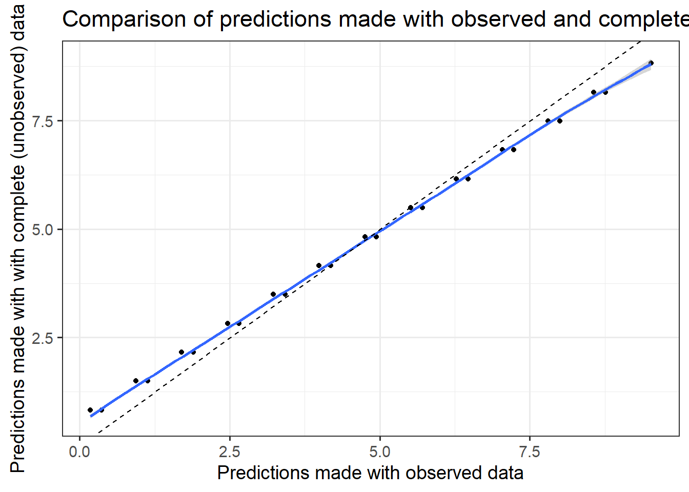
Now there is a difference between models fit on the observed data (with missingness) and models fit on a theoretically complete (no missingness) dataset. The linear model built using the observed data has biased parameters (intercept too high, slope too low).

f_p_bl <- function(age, n_zy, n_cl) {
    p_bl <- fifelse(n_cl >= 2, 0.8, 0.2)
    p_bl
}
df <- gen_data(1000,f_p_bl)
df1 <- make_observed(df)
miss_cl <- lm(n_cl ~ n_zy + age, data = df1)
true_cl <- lm(n_cl ~ n_zy + age, data = df)


miss_pred = predict(miss_cl,newdata=df1)
true_pred = predict(true_cl,newdata=df1)

res_df = data.table(miss_pred, true_pred)

ggplot(res_df,aes(x = miss_pred,y=true_pred)) + 
    geom_point() +
    stat_smooth() +
      labs(x= "Predictions made with observed data",
         y = "Predictions made with with complete (unobserved) data",
    title = "Comparison of predictions made with observed and complete data") +
    geom_abline(intercept=0,slope=1,linetype=2) +
  theme_bw(base_size=14)

`geom_smooth()` using method = 'gam' and formula = 'y ~ s(x, bs = "cs")'

References

Mohan, Karthika, and Judea Pearl. 2021. “Graphical Models for Processing Missing Data.” Journal of the American Statistical Association 116 (534): 1023–37.